What transmission line parameters R, L and C are, and why they matter

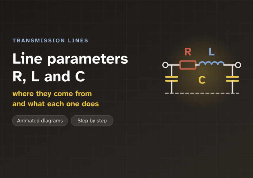
In this guide we follow current along one high-voltage line, with animated diagrams, and see where its resistance, inductance and capacitance come from and what each one does.

The problem: a line is more than a wire

On a single-line diagram, a transmission line is just one straight stroke. It looks like a perfect wire. But a real line is tens or hundreds of kilometres of metal, hanging in the air above the ground.

Along that length, the line has electrical properties of its own. They change the voltage and the current that reach the far end. We call them the line parameters. They are the fixed electrical values of the line, given per kilometre.

Two everyday results show this. With heavy load, the voltage at the far end sags. With no load on a long line, the far-end voltage can rise above the sending-end voltage. So how can one piece of wire do both?

The graph below shows the two cases. Voltage is given in per unit (pu). Per unit means a fraction of the rated value, so 1.00 pu is exactly the rated voltage.

The answer is three parameters, working at the same time. Resistance, inductance and capacitance. Each one has a clear physical cause, and each one does a different job.

What decides R, L and C

Most high-voltage overhead lines use ACSR conductor. ACSR means aluminium conductor, steel reinforced. A core of steel strands gives the strength. Layers of aluminium strands around it carry the current.

Resistance (R) is the opposition of the metal to current. It depends on the material, the length and the cross-section area. A popular conductor called "Drake" is 28.1 mm across. Its DC resistance is about 0.070 Ω/km at 20 °C. Hot, at 75 °C, its AC resistance is about 0.086 Ω/km.

Most of that rise comes from temperature. Aluminium resistance goes up about 0.4% for each degree. A small part comes from the skin effect, the way AC current crowds toward the outside of a conductor. For this size at 50 Hz, the skin effect adds only about 1%.

Inductance (L) and capacitance (C) do not depend on the metal. They depend on geometry. That means the conductor radius r, the spacing D between the phases, and the height h above ground. The figure below shows both views.

High-voltage lines often use a bundle. This is two, three or four sub-conductors per phase, held apart by spacers. A bundle behaves like one much fatter conductor. That lowers L and raises C. It also cuts corona, the faint electrical discharge that forms in the air around a highly charged conductor.

There is a fourth parameter, called conductance (G). It covers tiny leakage over insulators and corona loss. It is so small that we usually ignore it.

The core idea: two fields around every conductor

A live conductor carries two things at once. It carries current, and it sits at a high voltage. Each one makes its own field.

The current makes a magnetic field. It forms rings around the conductor. In AC, the current changes direction 50 times a second, so the field keeps growing and collapsing. A changing field pushes back on the current that made it. This push-back is the inductance.

Spacing matters a lot. Picture the current going out on one conductor and back on another. Between them is a loop. The magnetic flux trapped in that loop decides the inductance. Move the conductors apart and the loop gets bigger. It traps more flux for each amp. So L goes up.

The voltage makes an electric field. It reaches from the conductor to the other phases and to the ground. A conductor and the ground with air between them are just like the two plates of a capacitor. They store charge. This is the capacitance.

Here spacing works the other way. Plates that are far apart store less charge for each volt. So when D goes up, C goes down. The figure shows both effects side by side.

Notice one more thing. L and C move in opposite directions, but both follow the same term, ln(D ÷ r). ln means the natural logarithm. A logarithm grows slowly, so doubling the spacing changes L and C only by about 10%. That is why most overhead lines have similar values. A typical 400 kV line has L near 1.0 mH/km and C near 12 nF/km.

Move the slider to see this for yourself. Watch how slowly the curves bend.

The pill shows the reactance X. Reactance is the AC opposition caused by inductance, X = 2π × f × L, in ohms. The note also gives the surge impedance, √(L/C). It is the natural impedance of the line. Most overhead lines sit between about 250 and 400 Ω.

Step by step: from tower drawing to line model

Engineers turn a tower drawing and a conductor datasheet into a circuit model. It takes four steps. Each card shows one.

Two details make the formulas work on real three-phase lines. First, the three phases are not always equally spaced. So we use the GMD, or geometric mean distance. For phases a, b and c, it is the cube root of D_ab × D_bc × D_ca. Second, the inductance formula uses the GMR, or geometric mean radius, instead of the real radius. GMR is a slightly smaller radius that also counts the magnetic field inside the metal. For a solid round wire it is 0.7788 × r. For Drake, the datasheet value is 11.4 mm.

The formulas also assume a transposed line. Transposition means the phases swap positions at towers along the route. Each phase then sees the same average spacing, so the three phases stay balanced.

Step 4 gives the π model, named for its shape like the Greek letter π. R and L sit in series, in the path of the load current. Together they form the series impedance, Z = R + jX. C sits in shunt, from the line to ground. It forms the shunt admittance Y, the ease with which charging current flows to ground. We split it in half, one half at each end.

A worked example: a 200 km, 400 kV line

Let us put real numbers on a typical 400 kV line. Per kilometre, R = 0.03 Ω, L = 1.04 mH and C = 12 nF. The line is 200 km long and runs at 50 Hz.

Series values. R = 0.03 × 200 = 6 Ω. The reactance per kilometre is 2π × 50 × 1.04 mH = 0.33 Ω. So X = 0.33 × 200 = 66 Ω. X is about 11 times R. This is normal for high-voltage lines, and it is why L, not R, causes most of the voltage drop.

Charging current. The shunt susceptance is B = 2π × 50 × 12 nF = 3.77 µS per km, or 754 µS for the whole line. Susceptance is the AC "ease of flow" through a capacitance. The phase voltage is 400 ÷ √3 = 231 kV. So the charging current is 231 kV × 754 µS ≈ 174 A in each phase. It flows even when the far end is open.

Reactive power. The capacitance makes reactive power: V² × B = 400² × 754 µS ≈ 121 Mvar. Reactive power is the power that swings back and forth in the fields and does no useful work. It is measured in megavar (Mvar).

At 600 MW. The current is 600 MW ÷ (√3 × 400 kV) ≈ 866 A. The heat loss is 3 × 866² × 6 ≈ 13.5 MW, or about 2.3% of the power sent. The inductance uses 3 × 866² × 66 ≈ 149 Mvar of reactive power.

Look at the right chart. At this load, L uses a little more reactive power than C makes. They balance exactly at the surge impedance loading (SIL). For this line the surge impedance is √(1.04 mH ÷ 12 nF) ≈ 294 Ω. So SIL = 400² ÷ 294 ≈ 540 MW. Above SIL, the line uses reactive power and the voltage sags. Below SIL, C wins and the voltage rises. This is the Ferranti effect we saw at the start.

Where line parameters are used

R, L and C are inputs to almost every power system study. Load-flow studies use them to find the voltage at each bus and the power on each line. Short-circuit studies use the series impedance to find the fault current. Protection engineers set distance relays from the line impedance per kilometre.

The line length decides which model we use. A short line, under about 80 km, can ignore C. A medium line, from about 80 to 250 km, uses the π model above. A long line, above about 250 km, needs the exact distributed model. Engineers often write the result as ABCD parameters.

The parameters also explain cables. An underground cable has its conductors very close together, with solid insulation between them. A 400 kV cable can have about 0.95 µF/km, around 80 times an overhead line. Its charging current is huge. This is why long AC cables need shunt reactors, and why very long cable links often use HVDC instead.

Key takeaways

• A transmission line has three main parameters, spread along its length: resistance R, inductance L and capacitance C.
• R comes from the metal. It rises with length and temperature, and it is the only parameter that turns much power into heat.
• L comes from the magnetic field. Wider spacing gives more L. Its reactance X causes most of the voltage drop.
• C comes from the electric field. Wider spacing gives less C. It draws a charging current, even with no load.
• Typical 400 kV values are about 0.03 Ω/km, 1.0 mH/km and 12 nF/km. X is about ten times R.
• The π model puts R and L in series and splits C into two halves, one at each end of the line.